Материал: + An Orchestrated Survey on Automated Software TestCase Generation

came together, discussing application experience and tool support. Many of the academic conferences where general test automation work is published (like ICST, ICTSS (formerly TestCom/FATES), ASE, ISSTA, ISSRE, AST, etc.) regularly see a significant share of papers around MBT. Two Dagstuhl seminars have been conducted around the subject since 2004 (Brinksma et al., 2005; Grieskamp et al., 2011a); the report from the last event lists some of the open problems in the area. These all document a lively research community and very promising application area.

5. Test Data Generation in Combinatorial Testing

By Myra B. Cohen11

Combinatorial testing has become a common technique in the software tester’s toolbox. In combinatorial testing, the focus is on selecting a sample of input parameters (or configuration settings), that cover a prescribed subset of combinations of the elements to be tested. The most common manifestation of this sampling is combinatorial interaction testing (CIT), where all t-way combinations of parameter values (or configuration settings) are contained in the sample. In the past few years, the literature on this area of testing has grown considerably, including new techniques to generate CIT samples and applications to novel domains. In this section we present an overview of combinatorial testing, starting at its roots, and provide a summary of the two main directions in which research on CIT has focused

– sample generation and its application to di erent domains of

5.1. Introduction to Combinatorial Testing

software systems. Accepted

Throughout the various stages of testing, we rely on heuristics to approximate input coverage and outcomes. Combinatorial testing has risen from this tenet as a technique to sample, in a systematic way, some subset of the input or configuration space. In combinatorial testing, the parameters and their inputs (or configuration options and their settings) are modeled as sets of factors and values; for each factor, fi, we define a set of values, fx1; x2; :::xjg, that partition the factor’s space. From this model, test cases, or specific program configurations (instances) are generated, selecting a subset (based on some coverage criterion) of the Cartesian product of the values for all factors; a program with five factors, each with three values, has 35 or 243 program configurations in total. CIT has traditionally been used as a specification-based, system testing technique to augment other types of testing. It is meant to detect one particular type of fault; those that are due to the interactions of the combinations of inputs or configuration options. For instance,

11Acknowledgements: The authors would like to thank the anonymous reviewers for their helpful comments. This work is supported in part by the National Science Foundation through award CCF-0747009 and by the Air Force O ce of Scientific Research through awards FA9550-09-1-0129 and FA9550-10-1-0406. Any opinions, findings, conclusions, or recommendations expressed in this material are those of the authors and do not necessarily reflect the position or policy of NSF or the AFOSR.

10

if the aim is to detect faults due to combinations of pairs of configuration options, using combinatorial testing can satisfy this test goal using only eleven configurations.

The roots of combinatorial testing come from the field of statistics called design of experiments (Fisher, 1971; Cochran and Cox, 1957). In the 1930s, R.A. Fisher (1971) described a means to lay out crop experiments that combine independent variables in a systematic way, in order to isolate their impact

on the observed outcomes. In 1985, Mandl used these ideas to sampleManuscriptthe combinations of parameter values in compiler software through the use of orthogonal latin squares (Mandl, 1985).

Around the same time, Ostrand and Balcer (1988) developed the Category Partition Method, and the Test Case Specification Language (TSL), which gives us a way to model the factors and values so that they can be combined. In TSL, test inputs (or configurations) are modeled as categories and partitions, and for each a set of choices are described which are equivalence classes for testing. There are mechanisms to reduce the combinatorial space. Choices can be tagged as single, or error, or predicates can be defined that describe dependencies such as requires between elements. The full Cartesian product, that satisfy these constraints, is then generated.

In 1992 Brownlie et al. (1992) presented an extension of Mandl’s work called the Orthogonal Array Testing System, OATS, in which they used orthogonal arrays to define the combinations of an AT&T email system; all pairs of factor-values are tested exactly once. The work of Cohen et al. (1997, 1996) leveraged a key insight, that all factor-values must be tested at least once, lifting the exactly-once restriction of orthogonal arrays. This led to the use of covering arrays and the core underpinnings of combinatorial interaction testing (or CIT) as is used today. Out of this work came the Automatic E cient Test Case Generator (AETG), a greedy algorithm that generates covering array samples and includes both a modeling language and test process (Cohen et al., 1997, 1996).

Over the past several years we have seen a large increase in the number of algorithms for generating CIT samples and new applications that use CIT. We don’t attempt to provide a complete survey of CIT (for a recent survey see (Nie and Leung, 2011)), but instead provide a short overview and highlight some key research directions.

5.1.1. Example of CIT

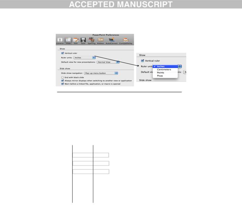
In Figure 2(a) we show the View preferences tab from a version of Microsoft Powerpoint. The user has seven configuration options that they can customize. Some of the configuration options such as Ruler units have multiple settings to choose from. We provide an enlargement of this selection menu which o ers the user the choice of Inches, Centimeters, Points or Picas in Figure 2(b). Other options such as End with black slide are binary; the user can select or deselect this setting. In total we have seven configuration-options, (factors) which we have shown as columns in the table (Figure 2c). The first factor, Vertical ruler, has two possible values, the second has four values, etc. In total, there are 2 4 3 24 or 384 unique configurations of View preferences. In practice this is only a part of the configuration space; if we combine this with the preferences from the Save

size (i.e. N) has been a focus of much work in this domain. While it is has been shown that the upper bound on the size of a covering array grows logarithmically in k (Cohen et al., 1997), it is non-trivial to construct CIT samples. Some instances of CIT construction have been shown to be NP Hard, such as finding the minimal size given forbidden constraints (Colbourn et al., 2004; Bryce and Colbourn, 2006).

5.2. Research Directions

The research on CIT has branched in two main directions. The first direction develops methods and algorithms to generate CIT samples, while the second direction refines CIT to work in novel application domains. We highlight work in each direction next.

5.2.1. CIT Generation

There is a long history of research on the mathematics of covering arrays which we do not attempt to cover, but instead refer the reader to two excellent surveys, one by Colbourn (2004) and another by Hartman and Raskin (2004). Mathematical techniques may be probabilistic (i.e. they do not construct, but prove existence of arrays), or provide direct constructions. Constructions are deterministic and produce arrays of known sizes, but are not as general as heuristic methods, known only on a limited subset of possible parameter settings for t, k and v. C. Colbourn maintains a website with references of known array sizes and associated techniques (Colbourn, 2012).

Heuristic techniques to generate CIT samples have domi-

nated the literature on CIT. The first algorithms were greedy, of which there are two Acceptedprimary types. One class follows an AETG-like mechanism (Cohen et al., 1997). Examples are the

Test Case Generator (TCG) (Tung and Aldiwan, 2000), Deterministic Density Algorithm (DDA) (Colbourn et al., 2004), and PICT (Czerwonka, 2006). One test case at a time is added (the test case that increases the number of combinations that are covered the most) and within each row, the algorithms greedily chose the next best factor-value for inclusion. The heuristics used to select the next best factor-value di erentiate these algorithms. Some newer variants of this algorithm, use metaheuristic search techniques (such as genetic algorithms, tabu search, or ant colony optimization) to optimize selection of the factors with-in a row (i.e. that part is no longer greedy), but still retain the one row at a time greedy step (Bryce and Colbourn, 2007). A similar type of greedy algorithm, the Constrained Array Test System (CATS) (Sherwood, 1994), was proposed around the same time as AETG. It too selects test cases one at a time, but full test cases are enumerated and then re-ordered, so that the earliest test cases provide the greatest value towards covering uncovered factor-values. A second class of greedy algorithms are of the form used in the In Parameter Order Algorithm (Tai and Lei, 2002; Lei et al., 2008). In IPO, the algorithm begins with some number of factors k0 k and expands the size of the covering array horizontally (by increasing k0) and vertically (by adding new test cases to the sample to complete coverage if needed).

Meta-heuristic search techniques have been used to generate CIT samples, working on the entire sample at once. Some

12

size of N, is chosen as a start. Guided by a fitness function, and a stochastic process to transition through the search space, di erent solutions are tried and evaluated, until a covering array either is found for that N or a time-out has occurred. N is then adjusted in subsequent iterations until the smallest array is produced. Simulated annealing, has been the most widely discussed meta-heuristic algorithm for constructing covering arrays (Cohen et al., 2003a,c; Garvin et al., 2011).

Other approaches include genetic algorithms (Stardom, 2001), tabuManuscriptsearch (Nurmela, 2004) and constraint solvers (Hnich et al., 2006).

Another primary direction for CIT research, has been generating samples that consider dependencies (or constraints) between factor-values, called Constrained CIT (CCIT). For example, in Figure 2, suppose that the Vertical Ruler is not visible when using Picas because this functionality is unsupported. We do not want to include this combination in our samples (it will render the configuration infeasible). In CCIT satisfiability solvers have been used to aid in the evaluation of legal combinations of factor-values. In the work of Cohen et al., standard meta-heuristic search algorithms and greedy algorithms for CIT have been tightly-interwoven with SAT solvers to achieve this goal. Calvagna and Gargantini (2009, 2010) and Grieskamp et al. (2009) use solvers as the primary method to generate the samples. And more recently Binary Decision Diagrams BDD’s have been employed as a way to generate CCIT samples (Segall et al., 2011).

5.2.2. CIT Application Domains

The original uses of CIT was for test case generation where the factors and their values are system inputs or parameters and each row of the covering array is a test case (Brownlie et al., 1992; Cohen et al., 1997, 1996; Dalal et al., 1998; Dunietz et al., 1997). CIT has also been applied to test protocol conformance (Grieskamp et al., 2009; Burroughs et al., 1994).

More recent work samples configurations to be tested (under which many test cases will be run) (Qu et al., 2008; Yilmaz et al., 2006; Kuhn et al., 2004; Kuhn and Okun, 2006; Fouche´ et al., 2009; Dumlu et al., 2011). One type of configurable system, a software product line, has been an area of active research on CIT (Cohen et al., 2006; Perrouin et al., 2010). Software product lines are systems of program families that have a well managed asset base and feature model; from which one can derive a CIT model (Cohen et al., 2006; Clements and Northrop, 2001). McGregor (2001) first suggested that products in an SPL could be sampled for testing using CIT. Cohen et al. (2006) described a mapping from a feature model to a relational mode. Perrouin et al. (2010) have more tightly integrated construction with the feature model. There has been recent work that explores the use of CIT when testing sequences (Kuhn et al., 2012; Yuan et al., 2011). In traditional CIT, there is no notion of order (any two columns of the covering array can be swapped as long as a mapping is maintained for the concrete test cases to be applied). In sequence-based CIT, each factor becomes a location within a sequence, and the values within each factor are repeated at each location. This has been used to test graphical user interfaces (GUIs) (Yuan et al., 2011) and devices (Kuhn et al., 2012).

CIT has also been used to characterize the configuration option combinations that are likely to be the cause failures through the use of classification trees (Yilmaz et al., 2006; Fouche´ et al., 2009). More recently, Colbourn and McClary (2008) present special types of covering arrays, called locating and detecting arrays for the purpose of directly isolating the causes. Another new direction for CIT is to tune the test process and coverage through the use of variable strength covering arrays (Cohen et al., 2003b), prioritization (Bryce and Colbourn, 2006; Qu et al., 2008, 2007) and incremental covering arrays (Fouche´ et al., 2009), where the size of t can vary, the order of testing is prescribed, or we generate increasingly stronger t by re-using existing tests from lower strength t when moving to higher t.

5.3. Conclusion on Combinatorial Testing

In this section we have presented an overview of combinatorial testing, defined the primary mathematical object on which this research is based and presented some research directions that are being pursued. This is a promising area of research for automated software test generation, with opportunities to enhance new domains of its application. Fruitful future research directions for generating CIT samples includes automated model extraction, adapting to model evolution, and developing techniques that re-use or share information between di erent test runs. In addition to applying CIT to novel application domains, an area of potential for improvement in this direction is the combination of program analysis techniques with CIT to refine the sample space, and to target specific interac-

6. Test Data Generation by Adaptive Random Testing

tions at the code (as opposedAcceptedto only the specification) level.

Empirical studies have shown that failure-causing inputs tend to form contiguous failure regions: consequently, non-failure- causing inputs should also form contiguous non-failure regions. Therefore, if previously executed test cases have not revealed a failure, new test cases should be far away from the already executed non-failure-causing test cases. Hence, test cases should be evenly spread across the input domain. It is this concept of even-spreading of test cases across the input domain which forms the basic intuition for adaptive random testing, a family of test case selection methods designed to enhance the failure detection e ectiveness of random testing by enforcing an even spread of randomly generated test cases across the input domain. This section provides a brief report on the state-of-the-art of adaptive random testing.

6.1. Introduction to Adaptive Random Testing

Random Testing (RT) is one of the most fundamental and most popular testing methods. It is simple in concept, easy to implement, and can be used on its own or as a component of many other testing methods. It may be the only practically feasible technique if the specifications are incomplete and the source code is unavailable. Furthermore, it is one of the few

13

testing techniques whose fault detection capability can be theoretically analysed. Adaptive Random Testing (ART) (Chen et al., 2010, 2004) has been proposed as an enhancement to RT. Several empirical studies have shown that failure-causing inputs tend to form contiguous failure regions, hence non- failure-causing inputs should also form contiguous non-failure regions (White and Cohen, 1980). Therefore, if previous test cases have not revealed a failure, new test cases should be far

away from the already executed non-failure-causing test cases. Hence,Manuscripttest cases should be evenly spread across the input domain. It is this concept of even spreading of test cases across

the input domain, which forms the basic intuition of ART. Antirandom testing (Malaiya, 1995) also aims at even spreading of test cases across the input domain. However, a fundamental di erence is that ART is a nondeterministic method and antirandom testing is in essence a deterministic method with the exception of the first test case which is randomly chosen. Another di erence is that anti-random testing requires testers to specify the number of test cases in advance, whereas there is no such a constraint for ART.

To facilitate discussion, it is first necessary to define some terminology. By failure rate, we mean the ratio of the number (or size) of failure-causing inputs to the number (or size) of the set of all possible inputs (hereafter referred to as the input domain). By failure patterns, we mean the distributions and geometry of the failure-causing inputs. By e ciency, we refer to the computation time required, with lower computation time indicating higher e ciency. Strictly speaking, e ciency should also include memory, but memory will not be considered in this section due to space limitations and the lack of implementation details such as the data structures used. By e ectiveness, we refer to the fault detection capability which can be measured by the e ectiveness metrics including P-measure, E-measure, F- measure, etc. The F-measure is defined as the expected number of test cases required to detect the first failure; the P-measure is defined as the probability of detecting at least one failure; and the E-measure is defined as the expected number of failures detected. A set of test cases is assumed when using P-measure or E-measure.

RT is a popular testing method and ART has been originally proposed as an enhanced alternate to RT. This section will focus on the state-of-the-art of ART from the perspective of using RT as a baseline. We will only compare ART to RT, and not compare ART to other testing methods. We are interested in the problem that when RT has been chosen as a viable testing method for a system, is it worthwhile to use ART instead?

As a reminder to avoid any confusion and misunderstanding, cost-e ectiveness in this section refers to the fault detection capability achieved for the resources spent. Some researchers (such as Arcuri and Briand (2011)) used the term “effective” where we use “cost-e ective”, therefore, when comparing across papers, such a di erence in the meanings should be noted. We decide to deal with e ectiveness and e ciency separately in this section because such an approach will give us a better picture about which aspect or direction shall be improved.

6.2. Various ART Algorithms

Various approaches have been identified to implement the concept of even spreading of test cases across the input domain. As a consequence, a number of di erent ART algorithms have been developed (Chan et al., 2006b; Chen et al., 2004, 2009, 2004; Ciupa et al., 2008; Lin et al., 2009; Liu et al., 2011; Mayer, 2005; Shahbazi et al., 2012; Tappenden and Miller, 2009). The major approaches include:

1. Selection of the best candidate as the next test case from a set of candidates. This approach first generates a set of random inputs as candidates from which the best candidate, as defined against set criteria, is selected as the next test case.

2. Exclusion. In each round of test case generation, this approach first defines an exclusion region around each already executed test case. Random inputs are generated one by one until one input is outside all exclusion regions of the already executed test cases, and then this input is selected as the next test case.

3. Partitioning. This approach uses the information about the location of already executed test cases to divide the input domain into partitions, and then to identify a partition as a designated region from which the next test case will be generated.

4. Test profiles. Instead of using a uniform test profile as normally adopted by RT, this approach uses a specially designed test profile which is able to achieve an even spread-

ing of test cases over the input domain. Dynamic adjust- Accepted

ment of the test profile during testing is required in this approach.

5. Metric-driven. Distribution metrics, such as discrepancy and dispersion, are normally used to measure the degree of even distribution for a set of points. Instead of being used as a measurement metric, this approach uses the distribution metrics as selection criteria to select new test cases such that a more even distribution of the resultant test cases could be obtained.

The above is not an exhaustive list, but rather gives some of the most popular approaches. Furthermore, it should be noted that for each approach, di erent methods can be used to achieve an even spreading of test cases. Therefore, many ART algorithms have been developed. For example, the most popular algorithm taking the first approach is the Fixed-Sized-Candidate-Set ART (hereafter referred to as FSCS-ART) (Chen et al., 2004) in which a fixed-size candidate set of random inputs is first generated whenever a new test case is needed. For each candidate set, a selection criterion is applied to select the best candidate as the next test case. Adopted selection criteria include maximin, maxi-maxi, maxi-sum, etc. For maxi-min, the distance (or dissimilarity in the case of non-numeric inputs) between each candidate and its nearest already executed test case is first calculated. The candidate with the largest such distance is then selected as the next test case. For maxi-sum, the distances between each candidate and all the already executed test cases are first summed. The candidate with the highest such sum is then

14

selected as the next test case. Intuitively speaking, inputs near the boundaries of the input domain will have a higher probability of being selected as test cases when maxi-min is used instead of maxi-sum. In other words, di erent ART algorithms have di erent e ectiveness performance, e ciency performance and characteristics which in turn give rise to di erent favourable and unfavourable conditions for their applications.

As FSCS-ART is the first published ART algorithm and has

been the most cited ART algorithm since the inception of ART, someManuscriptprevious studies have treated FSCS-ART and ART as equivalent or exchangeable. We would like to emphasize that

FSCS-ART is only one of the many members of the family of ART algorithms, and FSCS-ART is not equivalent to ART which refers to the family of testing methods in which test cases are random and evenly spread across the input domain. Obviously, the strengths and weaknesses of a particular ART algorithm for a specific type of software are not necessarily valid nor expected to be similar for other ART algorithms.

For numeric input domains, the distance (or dissimilarity) metric used to measure “far apart” is easily and naturally defined. However, the choice of a distance metric for non-numeric input domains may not be straightforward. We have proposed a generic distance metric based on the concept of categories and choices (Kuo, 2006; Merkel, 2005). Ciupa et al. (2008) have proposed a specific distance metric for object-oriented software. Tappenden and Miller (2013) have proposed a specific distance metric for cookies collection testing of web applications. It is understood that there are currently investigations into the application of ART in input domains involving strings, trees, finite state machines, etc.

6.3. E ectiveness

In the studies of ART, the adopted e ectiveness metrics include F-measure, P-measure and the time to detect the first failure. Obviously, di erent e ectiveness metrics have di erent strengths and weaknesses, and there is no single best e ectiveness metric. Also, it is common that a testing method is better than another testing method with respect to one e ectiveness metric, but worse if measured against another metric. Therefore, a metric may be appropriate in one scenario but inappropriate in another. The selection of an appropriate metric is in itself a challenging problem.

The F-measure has been the most frequently used metric to compare the e ectiveness of ART and RT. Chen et al. (2004) compared RT and ART using 12 open source numerical analysis programs written in C++, with seeded faults. For three out of these 12 programs, there was no significant di erence between the F-measures of ART and RT; for one program, the F- measure of ART was about 90% of the F-measure of RT; and for the remaining eight programs, the F-measure of ART was between 50% and 75% of the F-measure of RT. Ciupa et al. (2008) compared RT and ART using real-life faulty versions of objectoriented programs selected from the Ei eBase Library. Their results showed that the average F-measure of ART was about 19% of the F-measure of RT. Lin et al. (2009) compared RT and their ART using six open source Java software artifacts with seeded faults. The average F-measures for ART and RT were